
Multi Armed Bandit history
The concept of ranking specific content has been widely studied in the IR field through the Learning to Rank framework. Recent ranking trends seem to have blurred boundaries, and although deep learning models often involve batch learning/inference rather than real-time learning/inference, the need for Online Learning has been significant in the recommendation field, and there are still many cases where Online Learning to Rank is solved through the MAB framework.
I have briefly summarized how to define OLTR with the MAB framework and its history.
Mentioned MAB Algorithms
Classical MAB: $\epsilon$-greedy, UCB, Thompson Sampling
Contextual MAB: LinUCB (WWW 10), LinTS (ICML 13), GIRO (ICML 19)
Non-stationary MAB: DiscountedUCB + SlidingWindowUCB (ALT 11), CUSUM-UCB + PHT-UCB (AAAI 18), dTS (NIPS 17)
Contextual + Non-stationary MAB: NeuralBandit (ICONIP 14), dLinUCB (SIGIR 18)
Multiple Play MAB
-
Simple Solution: MP-TS + IMP-TS (ICML 15)
-
Combined with Click Model: CascadeUCB1 + CascadeKL-UCB (ICML 15), RecurRank(ICML 19)-Non MAB
-
Combinatorial Perspective: CUCB (ICML 13)
-
Combinatorial + Volatile arm: CC-MAB (NIPS 18)
Batched Update MAB: bTS (IEEE BigData 18)
Using Feedback as Relative Perspective: RUCB (ICML 14), CDB (RecSys 19)
Exploration-Exploitation Dilemma
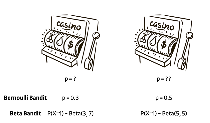
Suppose a single-armed bandit has the opportunity to pull two slot machines, and the two slot machines have different probabilities of returning a reward. How should you pull the slot machine to get the highest expected reward without knowing that?
The assumption used in Classical MAB is that the slot machine generally follows a Bernoulli distribution for the probability of returning a reward. Then, if you keep pulling the slot machine with a higher probability, you can get the best result. However, since we are not an oracle (knowing the probability or distribution), we need to explore which slot machine will return more rewards.
Here, the difference between the expected reward when making the best choice (the right slot machine in the picture) and the expected reward when not making the best choice is called regret. For example, in the picture above, a regret of 0.2 accumulates every time you pull the left machine. The way regret is defined varies from paper to paper, but it’s not an important point in real service applications, so you can just understand the concept and move on.
So, how do you define a reward in a recommendation system? If you define reward 1 as occurring after exposure (impression) and click, and no reward as occurring after unclick, the expected value of the reward becomes the expected value of clicks per exposure, and that becomes CTR!! Tada~~ Therefore, minimizing regret == maximizing CTR becomes the same.
In summary: We don’t know, but let’s find out by pulling.
Classical MAB
1. $e$-greedy
Of the traffic, $\epsilon$ is randomly explored, and the remaining $1-\epsilon$ is greedily drawn to the best arm based on the results observed so far, a strategy called $\epsilon$-greedy. As the trial continues, it is assumed that the estimate of the reward of the slot handle $a$ converges to the true value. However, in cases where the number of observations is small, the reliability of the observation results is very low, causing problems. (e.g., 12345 was recommended 4 times, and 3 was clicked twice, and 4 was clicked once. Is 3 the best case? Can you trust this result?) Conversely, even if the number of observations is sufficient and the reliability is high, the fact that you must explore at least $\epsilon$ is a problem. This problem can be solved by appropriately reducing the exploration probability over time. If you appropriately reduce the exploration probability, the regret $R_A(T)$ that occurs when you do not make the best choice at time T, divided by T, $R_A(T)/T$, will converge to 0.
2. Optimism in Face of Uncertainty (OFU)
OFU is an algorithm with the concept of looking optimistically at uncertainty. Like a rosy future is drawn after an investment
The previously explained $\epsilon$-greedy always chooses the arm with the good empirical mean and the rest with the probability of epsilon, but since the actual reward from the arm is not a constant but a r.v drawn from a specific distribution, the concept of confidence interval is introduced into the exploration strategy. OFU uses the upper confidence bound (UCB) calculated statistically based on the results observed so far as the value of that arm and draws that arm.
For example, when you have estimated the following posterior distribution based on the observed results, although the mean value is blue<green<orange in order, the upper limit of the 95% confidence interval is blue, so you draw the blue arm.

There are several modified algorithms depending on how UCB is defined, but the way the representative UCB algorithm UCB1 chooses an arm is as follows.
\[i = \underset{i}{argmax} \bar{x_i}+\sqrt{\frac{2lnt}{n_i}}\]$x_i$ is the average value of the observed rewards (clicks) for the i-th arm, and $n_i$ represents the number of times arm i has been played (impression). The above value represents the upper bound of the $1-\frac{1}{t}$ confidence interval for the actual reward of arm i, which is obtained by the Chernoff-Hoeffding bound. Initially, arms with fewer observed results are more likely to be selected (exploration), but as time increases on a log scale and $n_i$ increases linearly, the value of the right-hand side decreases over time, reducing the proportion of exploration as time passes.
3. Thompson Sampling
Also known as Probability Matching. It’s an algorithm used in Google Analytics for A/B testing optimization, and it generally shows higher performance than UCB or $\epsilon$-greedy. At time $t$, when arm $a$ is selected according to the policy, and the corresponding reward $r$ is received, Thompson sampling designs the likelihood function $P(r \mid a, \theta)$ using observations ($a_t,r_t$) and parameter $\theta$, and then solves for MAP (Maximum A Posteriori) assuming a prior. If each arm’s reward probability $\theta_k$ is assumed to follow an independent Bernoulli distribution, then due to the conjugacy property, if the prior is set as a beta distribution, the posterior will also be a beta distribution. At this time, $\theta_k$ has the following parameters:
\[\theta_k \sim Beta(\alpha_k, \beta_k)\]Since the distribution is assumed, the mean and variance can be known through the distribution. Here, the variance signifies Explore. The mean and variance of the beta distribution are as follows:
\[\begin{align} E[\theta_k] &= \frac{\alpha}{\alpha+\beta} \newline V[\theta_k] &= \frac{\alpha\beta}{(\alpha+\beta)^2(\alpha+\beta+1)} \end{align}\]Thompson Sampling’s parameter update occurs as follows, so as the trials repeat, the variance decreases, and the degree of Exploration diminishes. Here, $c_i \in {0, 1}$ signifies the presence or absence of a click.
\[\begin{align} p(u) &\propto \mu^{\alpha-1}(1-\mu)^{\beta-1} \; \newline Likelihood &= \prod_{i=1}^N \mu^{x_i}(1-\mu)^{1-x_i} \newline posterior &= likelihood \cdot prior \end{align}\]While the OFU algorithm makes decisions based on the upper confidence bound of the estimated distribution, the TS algorithm makes decisions by directly sampling from the estimated distribution.
The video below implements Thompson Sampling in a Bernoulli bandit and simulates it. You can observe the process of fitting a beta distribution in a bandit situation where the probability of observing a reward in each bandit is $\theta=[0.1,0.2,0.3,0.4]$ and $K=4$. At the same time, you can observe the degree of Exploration-Exploitation.
After Classical
Instead of thoroughly reading a single paper, I aimed to broadly understand the trends in MAB research.
What I felt while conducting MAB research is that most sota papers conduct experiments using existing MAB methodologies as baselines, claiming better performance than them. However, since most MAB papers assume ideal situations like stationary, Top-1 draw, reward ~ R-sub Gaussian, I highly doubted whether the performance improvement in papers introducing SOTA algorithms, especially in offline evaluation situations, would actually occur when applied to real services. I focused my research on what are the limitations that SOTA algorithms are trying to overcome from existing algorithms? because I think that summarizing the concepts of various algorithms will help in faster problem-solving later on.
1. Non-stationary MAB
Classical MAB destroys the assumption that the reward distribution is time-independent. As time passes, the expected CTR of a specific arm can decrease or increase. Non-stationary environments are defined as Slowly-varying, where the expected value of the reward changes gradually, and Abruptly-changing, where consistency is maintained before and after the breakpoint, and MAB policy is also divided into two major categories to suit each environment.
1.1. Passively Adaptive Policies
By using the concept of time discounting and giving higher weight to recent data, you find the current best arm. In this category, ofu methods include DiscountedUCB, SlidingWindowUCB, and based on Thompson sampling, there is discounted Thompson Sampling (dTS) introduced in Taming Non-stationary Bandits: A Bayesian Approach (NIPS 2017).
DiscountedUCB uses gamma to discount past observation results over time, reducing their influence, and SlidingWindowUCB uses only the observation results for a specified window period. These passive adaptation methods reduce the influence of past data but do not eliminate it, leading to a Time-lag problem where they cannot respond quickly to sudden changes.
1.2. Actively Adaptive Policies
A Change Detection Algorithm is used to quickly detect abrupt changes. Two-sided CUSUM UCB, PHT-UCB were introduced in A Change-Detection based Framework for Piecewise-stationary MAB Problem (AAAI 2018). Among them, Two-sided CUSUM UCB uses the CUSUM control chart, a statistical process control (SPC) change detection model used mainly for Fault Detection, and PHT-UCB uses the Page-Hinkley Test for change detection.
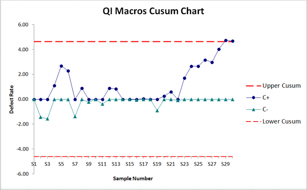
When the model sends a change detection signal to UCB or LCB of CUSUM or PHT Chart, the bandit algorithm is reset, and retraining is carried out. The structure is as follows:

Algorithms considering non-stationary environments in contextual bandit situations include NeuralBandit introduced in A Neural Networks Committee for the Contextual Bandit Problem (ICONIP 2014), and dLinUCB introduced in Learning Contextual Bandits in a Non-stationary Environment (SIGIR 2018).

The dLinUCB algorithm updates multiple slave bandit models simultaneously, discards old models based on the confidence interval of the reward, and re-trains them, using the currently optimal model in a unique way. It proposes a unique structure that can ensemble multiple models because the slave models do not have to be one type of LinUCB.
2. Context-Reward Relationship
In the case of a slot machine, the probability of observing a reward is fixed, but in actual services, the probability of observing a reward can vary depending on the surrounding environment or users. If so, assuming that the distribution of rewards follows a Bernoulli distribution regardless of the context can also lead to a critical problem.
Attempts to reflect the distribution of rewards by combining information not used in the existing MAB scheme, such as context and feedback feedback, were made through contextual bandits. LinTS and LinUCB assume that the expected value of the context and reward of the user (query) and content has a linear relationship, and are used to learn the expected value of the reward using not only feedback but also context information. Also, both algorithms update ridge regression parameters in Closed Form without using methods like SGD.
However, one may question the basic assumption of LinTS and LinUCB that the expected value of context and reward has a linear relationship. NNBandit (ICONIP 2014) is a model that represents the non-linear relationship between context and the expected value of reward by utilizing the fact that Neural Net is a Universal approximator.
In addition, solutions such as GLM, Balanced linear model, Adaptive learning, and Bootstrap have been proposed. The more complex the model, the more naturally it captures the context-reward relationship, but since this operation must be performed for all arms of the bandits, even a slight increase in computational load can significantly increase the actual execution time. If it’s not in linear form, updates must be performed using SGD or Mini-Batch methods in online learning situations, so you must choose a model that fits the situation considering computational resources.
3. Multi-play
The “multi” in Multi-armed bandit assumes that there are K arms, but it assumes a single play situation where only one arm can be pulled at a time. However, in real services, there are definitely cases where you have to draw several at once from the K arms, like an octopus.

If you only draw (impression) one and click on this recommendation result, you give a reward value of 1 or 0, but it is necessary to question whether it is reasonable to update the reward in the same way when drawing several (best L) at once. This is because the reward is not observed with a probability of $\theta_k$ independently in each arm, but there is a constraint that a maximum of one reward is observed.
3.1 Simple Idea
Optimal Regret Analysis of Thompson Sampling in Stochastic MAB Problem with Multiple Plays (ICML 2015) introduces a way to deal with multi-play situations. The MP-TS proposed in this paper is virtually no different from TS, but in multiple-play situations, it performs Beta draw to draw the top-L instead of the top-1, and updates the reward of 1 or 0.
At the same time, it proposes I(mproved)MP-TS as an improved version of MP-TS, stating that suboptimal draws occur too often, so L-1 of the L slots will give the best results from previous observations (exploitation), and only one will perform Beta draw of existing Thompson sampling (Exploration).
This method is reasonable if all the drawn arms have independent Expectation rewards, but reality is not. Among the L exposed contents, there may be people who have not even looked at the exposed content from n+1 after clicking on the n-th content, and the 3rd exposed content may affect the 4th exposed content click. Also, even if all L are liked, only one click can be made.
3.2 Click Model
Such research led to attempts to solve the problem by combining Click Model, which analyzes user behavior patterns in the IR field, with MAB, and the representative Click Models are as follows. (Reference: Click Models for Web Search (Authors’ version))
Notation
$u$ : document id
$q$ : user’s query
$u_r$ : A document at rank r
$C_u$ : r.v for Click document u
$E_u$ : r.v for Examinate document u
$A_u$ : r.v for Attractiveness of document u
$S_r$ : r.v for Satisfaction level after click
- Random Click Model (RCM)
The most basic CTR prediction model assumes that all content has the same click probability $\rho$. The Classical MAB is based on this assumption.
- Rank-Based CTR Model (RCTR)
This model assumes that the expected value of CTR varies depending on the order (rank) in which the content is exposed. It is a considerably realistic baseline model, and in the user behavior pattern study of Accurately interpreting clickthrough data as implicit feedback (SIGIR 2005), the CTR of Rank 1 content was observed to be 0.45, while the CTR of Rank 10 content was lower than 0.05. The actual in-house click model also shows similar CTR depending on the position, consistent with the experimental results.
However, this Click ratio cannot be directly applied to the RCTR model, as the actual slot-specific CTR is influenced not only by the effect of rank but also by the effect of MAB’s effort to find the best rank.
- Position-based Model (PBM)

The CTR of PBM can be represented by the Bayesian Network above (see: PRML-Bayesian Network). This model assumes that a click occurs when the user $q$ examines the recommended content (Examine) and is attracted to it (Attracted). In this model, the examination and attraction are assumed to be independent, with the examination influenced by the rank of content $u$, and the attraction influenced by both user $q$ and content $u$. Therefore, the Bayesian network is expressed by the following equations:
\[\begin{align} P(C_u=1)&=P(E_u=1)\cdot P(A_u=1) \newline P(A_u=1) &= \alpha_{uq} \newline P(E_u=1)&=\gamma_{r_u} \end{align}\]- Cascade Model (CM)
Introduced in An experimental comparison of click position-bias models (WSDM 2008), the CM is the most widely used assumption of user behavior patterns. It assumes that the user scrolls from top to bottom until they find the relevant content. The Bayesian network representing this is shown below.

In the CM model, the first recommended content is always examined, and the $r$-th content is examined only if the $r−1$ -th content is examined and not clicked. The equations are as follows:
\[\begin{align} C_r=1 &\leftrightarrow E_r = 1 \; and \; A_r=1 \newline P(A_r=1) &= \alpha_{u_rq} \newline P(E_1=1) &= 1 \newline P(E_r=1 | E_{r-1}=0) &= 0 \newline P(E_r=1 | C_{r-1}=1) &= 0 \newline P(E_r=1 | E_{r-1}=1, C_{r-1}=0) &= 1 \end{align}\]There are also various click models such as DCM.
These click models are used for slot-specific CTR prediction, and attempts to combine click models and MAB are made in Cascading Bandits: Learning to Rank in the Cascade Model (ICML 2015) due to the characteristic that these models reflect actual user behavior patterns well with Eye Tracking and HCI-based research. This includes the combination of the most widely used Cascade model and MAB, with CascadeUCB1 and CascadeKL-UCB introduced in the paper.
Also introduced is BC-MP-TS (Bias-Corrected MP TS), a modification of MP-TS to solve the bias that arises in the Cascade situation, as mentioned in the paper that introduced IMP-TS.
The contextual versions of these models, CascadeLinTS and CascadeLinUCB, were introduced in Cascading Bandits for Large-Scale Recommendation Problems (UAI 2016).
3.3 Combinatorial Bandit
Combinatorial bandit is a bandit algorithm that takes a broader perspective than using a click model.
The paper that led to active subsequent research on this bandit algorithm is Combinatorial MAB: General Framework, Results and Applications (ICML 2013). If Cascade Bandit is suitable for the IR field, where multiple clicks can occur in the same recommendation result by arranging recommendations in a Vertical manner, the Combinatorial method introduces the concept of Super arm, making it more versatile and suitable for deriving strategies in multiple-draw situations in recommendation systems.

In situations where multiple arms must be drawn, and there is a correlation between arms, the legitimacy of estimating the absolute value of individual arms wavers. Therefore, the combination of arms drawn together is defined as a super arm.
Simply put, if you treat all possible super arms as individual arms, you can solve the problem using the existing Classical 1-draw bandit method. However, if there are $m$ arms, the possible super arms are a maximum of $2^m$, and in a situation where L arms are drawn, $_mC_L$, exponentially increasing compared to the number of existing arms, so you cannot solve the problem in this way.
Therefore, the paper proposes creating an oracle function to form appropriate combinations of arms. The oracle function varies from paper to paper, but it constructs an Expectation vector of individual arms (underlying arms) based on the observed draws and reward data, and uses this vector to form the optimal combination of arms, the super arm. How the mapping is done is the most crucial part, and the paper constructs the super arm through $\alpha,\beta$-Approximation, and Efficient Ordered Combinatorial Semi-Bandits for Whole-Page Recommendation (AAAI 2017) defines the Maximization problem instead of Oracle, and calculates it through the following network structure for computational efficiency.

It’s regrettable that I started studying Combinatorial Bandit late and couldn’t organize it more, but Contextual Combinatorial MAB with Volatile Arms and Submodular Reward (NIPS 2018) introduces the CC-MAB algorithm, a combinatorial bandit algorithm that considers the situation where the pool of available arms is continuously changing (volatile arms).
4. Batched Update
A Batched Multi-Armed Bandit Approach to News Headline Testing (IEEE BigData 2018) is a study conducted by Yahoo Research. MAB assumes that drawing an arm and updating the reward occurs sequentially and immediately on an event-by-event basis. However, in real services, traffic comes in at a very fast pace, and the bTS (batched Thompson Sampling) algorithm is proposed to consider situations where it can only happen in batch units.
In this paper, methods of updating the parameters of the beta distribution through summation and normalization were proposed. The normalization update method is proposed to solve the side effects caused by traffic being concentrated in batch units.
\[\begin{align} \alpha_{t+1} &= \alpha_{t} + c_t \newline \beta_{t+1} &= \beta_{t} +u_t \end{align}\][Summation] $c_t$: clicks in batch t, $u_t$: unclicks in batch t
\[\begin{align} \alpha_{t+1} &= \alpha_{t} + \frac{M_t}{K}\frac{c_t}{c_t + u_t} \newline \beta_{t+1} &= \beta_{t} + \frac{M_t}{K}\left ( 1 - \frac{c_t}{c_t+u_t} \right ) \end{align}\]
[Normalization] $M_t$: the number of impressions of all arms in batch t, $K$: number of arms
However, the experimental results in this paper showed that the summation method performed much better. The authors analyzed that the effect of noise occurring during normalization update seemed greater than the effect of handling side-effects.
5. Is the Value of an Arm Absolute? (OLTR)
This time, it’s a problem raised in a broader framework. In the Top L from N problem, the basic assumption of MAB is that each arm has an absolute value (expected value of reward). A brief investigation was also conducted into the method of solving the Online Learning to Rank (OLTR) problem without using this assumption.
Learning to Rank has its roots in the IR field. While the MAB method of online learning is widely used in recommendation systems, the IR field has compared other methods and the MAB method of learning to rank in the following paper: Online Learning to Rank: Absolute vs Relative (WWW 2015).
The Absolute approach refers to the general contextual bandit, synthesizing information from the document context, query, and user context to form context features and using this to estimate the absolute value of user feedback data (CTR in the MAB method).
However, the Relative approach questions the existence of the absolute value of specific content itself. It thinks that the information obtained from user feedback data in a situation where multiple recommendation results are exposed is not the absolute value of the content but only the relative preference between the exposed contents. Models corresponding to this relative approach learn ranking by updating user feedback using the Stochastic Gradient Descent method.
In the above paper, LinUCB was modified to Lin-$\epsilon$ and compared with the Candidate Preselection(CPS) Learning to Rank algorithm. In cases with a small number of user queries and documents (arms), and no noise in feedback, the MAB methodology showed better performance. However, when there was a lot of noise in user feedback or a wide range of the pool, the Relative approach (LTR) showed better performance.
There have also been attempts to combine this Relative approach with the Bandit algorithm, and the Bandit algorithm in this field is called Dueling Bandit. Relative UCB for the K-Armed Dueling Bandit Problem (ICML 2014) introduces the RUCB algorithm, which combines a relative interpretation that represents the relative preference from a pair of arms from the feedback information, and Online Learning to Rank for Sequential Music Recommendation (RecSys 2019) introduces the CDB algorithm.
The LTR field is too broad, so I couldn’t investigate in more detail, but Online LTR for Information Retrieval, conducted as a tutorial at SIGIR 2016, covers LTR in the IR field, especially Online LTR, in detail, so it would be good to read. I plan to read more and summarize it if I have the opportunity.

Do We Really Start from Nothing (無)?
The fundamental assumption of the Exploration, Exploitation dilemma is that we explore and find out by exposing first because we don’t know how the actual exposure results will turn out. So, do we really start from a state where we don’t know at all how the exposure results will be?
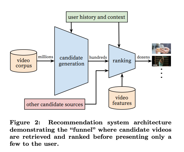
(출처: Deep Neural networks for YouTube Recommendations (Recsys 16))
In the general recommendation system structure, there are Scoring and Ensemble stages between Candidate Generation and Ranking (sometimes referred to as quality assessment models). If the scoring has a high correlation coefficient with the reward in the online situation, you can simply use that score as an initial value. Nowadays, well-refined features are available, and as models continue to evolve (deep! deeeeeep!), more precise pre-CTR Prediction is possible. Therefore, you can reduce the cold start problem of MAB by using the offline model’s CTR prediction as the initial value for MAB (e.g., setting the initial parameters for content A in Thompson Sampling to $\alpha=1$, $\beta=9$ if the CTR prediction for content A in the deep model is 0.1).
Comments